Polar map, Apex and distorted polar plot

Polar map, polar plot, contour plot

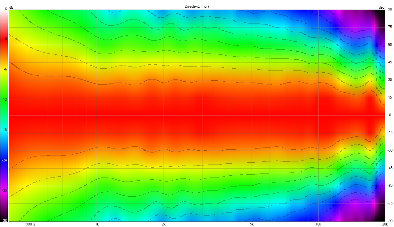
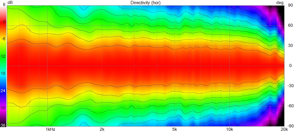
Heavily used at AudioHorn, the polar map or in fact the contour plot in our case, is a graphic representation of the energy radiation provided by a device, in dB scale versus angle in degrees.

It obtained by measuring the speaker, far away from reflective surfaces including floor, every 5 or 10° on an vertical axis by turning the speaker on itself, not moving the mic, at a precise distance and with gated measurements.

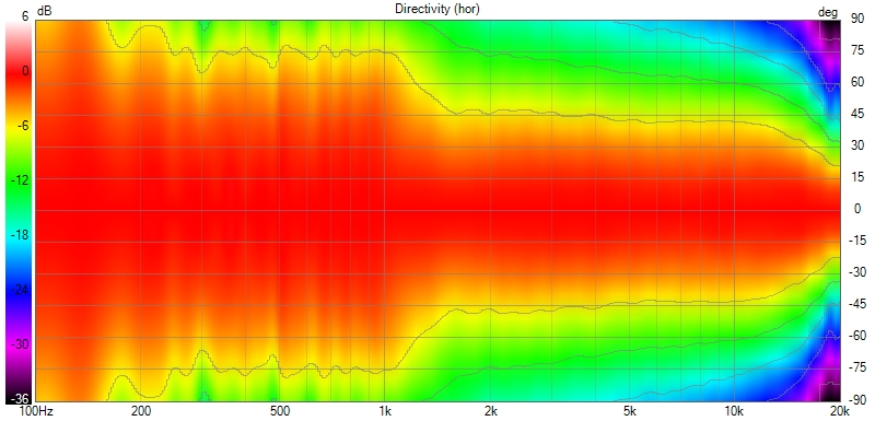
The contour plot has the advantage to make all the frequencies visibles in one graph:

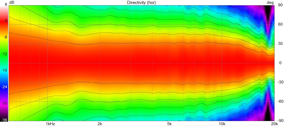
Where the -6 dB, here the transition from red to yellow by convention, defines the opening angle of the horn or waveguide.

As it’s flat we can also said that the directivity is constant, we use VituixCAD for visualization here.

But turning the speaker on itself means precisely using an axis, and to define where it is?

It’s why we will talk about Apex or apparent Apex.

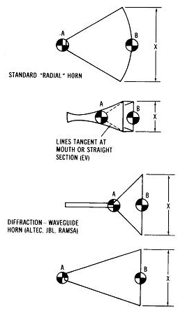
What is Apex ?

The apex is a point where the horn or waveguide’s profile axes virtually meet. In curved profiles, which are systematically used today (including in our designs), it corresponds to the intersection point of the geometric axes used to define and calculate the profile.

It is a practical virtual reference point, located near the horn geometry, used to describe the apparent origin of the radiated wave once it has been transformed by the horn.

Using this point as the rotation axis allows a near-field polar measurement, typically at 1 m or 1.5 m, to reproduce the same directivity representation as a far-field measurement at a greater distance, such as 3 m. If the apex is not respected, a so-called directivity distortion appears: the polar response changes with distance, leading to divergences as measurements are taken closer to the speaker.

The apex is not the acoustic source of the system, although in some designs both may coincide by choice. It is also often different between the horizontal and vertical planes.

In the case of polar measurement of a single element, we will place the mic at the height of the targeted element and rotate around the apparent apex.

This principle applies to horns and waveguides, but also to cone drivers, coaxial drivers and other transducers with an identifiable apparent Apex.

Horn and waveguide Apex

The Apex provides the appropriate reference for directivity measurements of a horn or waveguide.

Rotating around something other than the apex for a horn or waveguide will introduce a “distorted polar plot”: The closer we measure, the larger the mouth and deeper the apparent apex is, the more crucial this point is.

In the diagram below, point A represents the apex, while B is considered as the baffle reference:

This point allows to properly characterize a transducer (waveguide, horns but also coaxial or woofer driver) to have real directivity measurement.

Woofer Apex

The same principle applies to cone drivers, although the apparent Apex is often overlooked. In the upper part of a woofer’s operating range, the Apex is not located at the dust cap or at the baffle plane: it is a geometric point behind the diaphragm, determined by the cone profile.

For some woofers, it can be surprisingly far behind the front of the driver, sometimes on the order of twice the effective cone height. This becomes relevant when measuring directivity at short distances, typically around 1 m, where rotating around the baffle rather than the woofer’s Apex can produce a measurable distortion of the polar pattern.

Apex of a complete loudspeaker

This also explains why, in a complete loudspeaker using a waveguide or horn, the Apex of the woofer and that of the upper guided section can sometimes be very close or even practically aligned, despite their physical acoustic sources being separated.

For example, with the AudioHorn X-Shape 40 using a 15NTLW3500 woofer, the woofer Apex is approximately 16 cm behind the baffle, while the X-Shape Apex is also located approximately 16 cm in front of the compression driver, resulting in nearly coincident Apex positions.

This makes it possible, in this particular example, to measure the woofer and horn separately using essentially the same rotation axis, and then measure the complete loudspeaker around that same reference point.

When measuring a complete loudspeaker at close range, when the different elements do not have coincident Apex positions, a common reference should be chosen as close as possible to the median position of the different Apexes.

In practice, the Apex positions are generally not very far apart, so the midpoint between the woofer and upper-section Apexes is usually a very good reference.

This also applies to direct-radiating loudspeakers. A non-guided tweeter generally has an Apex close to its physical position, while a cone driver has its Apex well behind the front of the baffle. The baffle is therefore not necessarily a good common reference for the complete loudspeaker.

In an anechoic chamber, a complete speaker is typically measured around 3m (Don Keele), where the differences between the different Apex positions have a much smaller impact.

Acoustic center

The Apex is a geometric reference for the directivity of the individual sources and guided sections described above. At higher frequencies, where the wavelength is small compared with the relevant dimensions of the radiating structure, its geometry remains the relevant reference for directivity, with the Apex defining the corresponding measurement geometry.

At lower frequencies, however, the radiation of the complete loudspeaker needs to be considered differently. As the wavelength becomes large compared with the dimensions of the loudspeaker, the system progressively behaves more like a compact source and is better described in terms of an acoustic center.

The acoustic center is determined by the geometry and acoustic behavior of the complete system. It is influenced by factors such as the shape of the diaphragm and the geometry of the baffle or enclosure. It is therefore an acoustic property of the complete system rather than a fixed geometric point.

Its position varies with frequency. This also affects the measured phase and SPL, particularly at low frequencies, so the measured response can depend on the measurement distance.

From geometric Apex to acoustic center

As frequency decreases, the geometric Apex progressively becomes a less appropriate description of the radiation. When the wavelength becomes large compared with the dimensions of the driver and cabinet, the loudspeaker increasingly behaves as a compact source, and the relevant reference becomes the acoustic center described by Henwood and Vanderkooy.

This center is an acoustic property of the complete loudspeaker, not simply of the driver, and should not be confused with the acoustic or emission center used for time alignment between drivers.

There is therefore a gradual transition from the geometric Apex at higher frequencies to the acoustic center at low frequencies, rather than a precise frequency at which one suddenly replaces the other.

Henwood and Vanderkooy show that polar plots pivoted around the acoustic center exhibit much more consistent low-frequency behavior.

What determines the acoustic center?

Its position depends on factors including the piston size, baffle size and cabinet depth, and can be located several centimetres to several tens of centimetres in front of the baffle in typical low-frequency systems.

For some typical loudspeaker configurations, Vanderkooy gives a position of about two-thirds of the baffle radius in front of the enclosure. This corresponds to about one-third of the baffle diameter.

Merlijn van Veen’s acoustic center calculator can be used to determine both the frequency range where the acoustic center becomes the dominant reference and its corresponding position. It therefore provides a more precise frequency-dependent view of the transition, rather than simply referring to the typical region around 200 Hz.

The presence of a bass-reflex port can further complicate its position and behavior.

The acoustic center is therefore not a fixed geometric point of the enclosure, but a frequency-dependent description of the low-frequency radiation of the complete system.

As frequency decreases, this acoustic center moves progressively outward from the enclosure.

Acoustic center and horns

For HF and midrange horns and waveguides, the geometric Apex remains the appropriate reference throughout their normal operating range. These horns are generally not used at frequencies where the wavelength becomes larger than their mouth dimensions, so the acoustic-center description does not replace the geometric Apex in their intended operating range.

The situation can be different for low-frequency or kick horns. These larger horns can be used at frequencies where the wavelength becomes way larger than the mouth dimensions. As the source becomes acoustically compact, the acoustic-center description progressively becomes more relevant.

Low-frequency measurements

For a complete loudspeaker, the transition from the geometric Apex to the acoustic center is progressive and depends on the dimensions and operating range of the system.

For typical loudspeaker systems, the acoustic-center description has clear significance down to the region around 200 Hz, although the exact transition depends on the geometry of the system.

Below roughly 200 Hz, the acoustic-center description becomes increasingly dominant, and the geometric Apex of the woofer is no longer an adequate fixed reference for describing the radiation.

In addition, in a normal room, directivity measurements in this frequency region become progressively less useful because the acoustic field is increasingly dominated by room modes rather than by simple free-field radiation.

Note: The acoustic center can be useful for understanding low-frequency radiation and for obtaining coherent polar measurements, but it should not be interpreted as a reason to position a loudspeaker according to this point. At these frequencies, room dimensions, modal behavior and the distances to the walls have a much greater influence on the resulting response in the listening room.

And the temporal acoustic center?

At low frequencies, the acoustic centre also has a temporal meaning. When the loudspeaker behaves as an acoustically compact source, it can be represented as a monopole whose effective origin is the acoustic centre. The propagation time therefore corresponds to radiation originating from this effective point.

This is fundamentally different from the geometric Apex, which is a reference used to define the rotation axis for directivity measurements and does not represent the temporal origin of the acoustic wave.

As frequency increases, the compact-source approximation progressively ceases to apply, and the effective temporal origin moves back towards the actual radiating structure. It does not simply switch back to the Apex. The Apex remains a geometric reference for directivity, particularly for horns and waveguides, and should not be interpreted as their temporal acoustic centre.

Klippel Near-Field Scanner

The Klippel Near-Field Scanner (NFS) uses a fundamentally different approach from a conventional polar measurement.

Instead of rotating the loudspeaker around a fixed axis and keeping the microphone at a fixed position, the NFS keeps the loudspeaker stationary and moves the microphone around it, measuring the sound field at a large number of precisely known positions.

The important point is that the NFS does not simply measure a polar response at different angles. The exact 3D position of the microphone is known for every measurement point, allowing the system to capture the spatial distribution of the sound field in the near field.

The near-field measurements are then processed using a spherical wave expansion, based on spherical harmonics and Hankel functions, to reconstruct the radiated sound field. From this mathematical model, the sound pressure can be calculated at points outside the scanning surface, including in the far field.

This is fundamentally different from simply moving a microphone manually around a loudspeaker and treating the resulting measurements as a conventional polar plot. The NFS uses the spatial information contained in the complete set of measurement points and the mathematical reconstruction of the sound field to extrapolate the radiation into the far field. This allows the system to derive polar maps, directivity data, sound power and other far-field characteristics without performing a conventional far-field measurement at several metres.

The NFS therefore does not require the loudspeaker to be physically rotated around its Apex. The apparent Apex problem described above is specific to the conventional method, where the loudspeaker is rotated around a fixed point that defines the rotation axis.

This also means that the NFS can measure a complete loudspeaker system without having to determine a single mechanical rotation axis between the different drivers. The 3D spatial measurement and subsequent field reconstruction provide the information needed to model the radiation from the complete source.

The result is therefore not simply a collection of angular measurements. It is a reconstructed sound field from which the response can be calculated at different distances and angles in 3D space, including the far field.

It should not be reproduced manually: moving a microphone around a loudspeaker in a standard setup does not reproduce the NFS measurement. Without the precise spatial measurement and the subsequent spherical wave reconstruction, the resulting measurements cannot simply be treated as equivalent polar data.

What can distort a polar plot?

The distorted polar plot is not a distortion in the usual sense in audio, it should be seen as a trigonometric error between the position of the microphone, the apex and the width of the horn mouth.

The overall shape of the directivity will generally remain recognizable, but the opening given by the angle at -6dB will be in the wrong position, sometimes to a large extent. We are talking about a difference of the order of 10°. The entire energy distribution is therefore shifted and distorted.

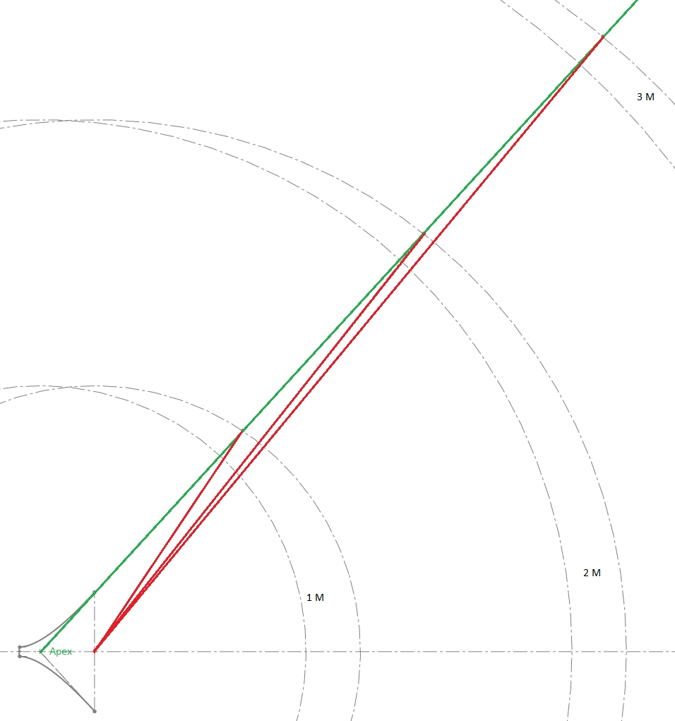
Here the green line is aligned with the opening of the horn and also shows how to find the Apex and the red lines are the equivalent by rotating around the baffle, but this is valid at any point.

Note: A horn is never measured free-air without full roundover or ISO baffle, if not a lot of midrange narrowing will appear.

We can see on this diagram that the further from the DUT (Device Under Test) we are, the smaller the difference is between rotating arround the baffle compared to rotating arround the APEX.

So in a close measurement of a large horn, the rotating axis must be close to the horn’s Apex.

Gated measurements

Even if you measure at 1m of the Apex you will have a floor/ceiling bounce that will impact your measurement in the lower range, you can visualize it with a tool in VituixCAD to see when (in time), according to distance and height position of elements, you will have it.

The way to do is: In your measurement tool, usually REW, you have to look at the Impulse, check where the accidents due to surfaces occur in time and then gate the measurement just before the first accident as shown here:

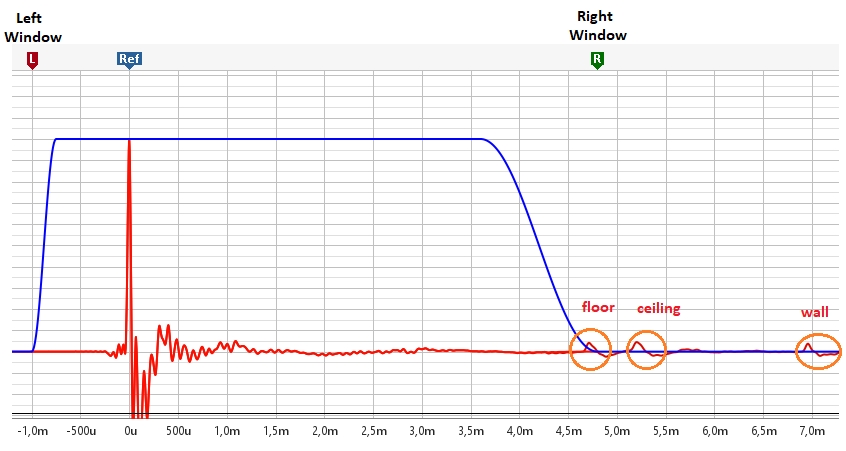
Here we put:

Lef Winfow: 1ms
Right Window: 4.8ms, just before floor reflection

Be also sure that Ref is on the impulse of the driver because at 75 or 90° the wall reflection can be more important in volume than the driver itself due to the fact that we turn the speaker or horn.

So the measurement tool can in some cases choose the wrong Ref and put it on a reflection, so we have to move the ref to the real driver impulse, to the left.

A gated measurement suppresses reflections arriving after the selected time window, but the shorter the window, the poorer the low-frequency resolution and the higher the lowest reliable frequency. For low or midrange horns, the horn must be moved further away from reflective surfaces to extend the time before reflections enter the window.

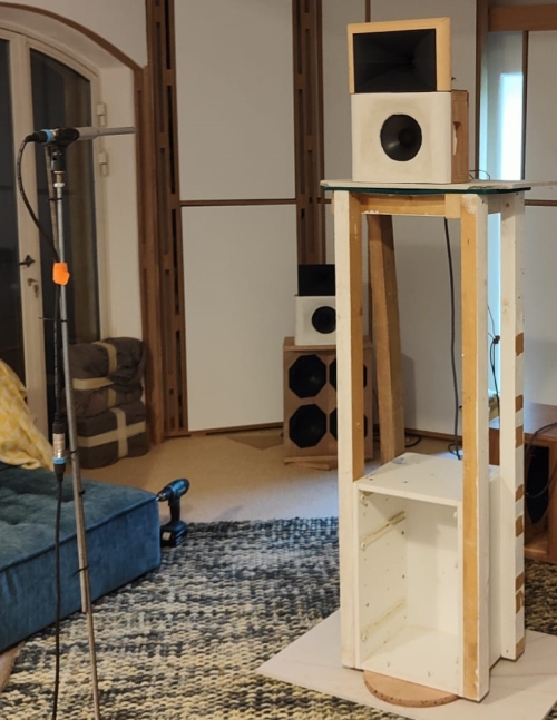
Important: When measuring and then gating a high-frequency horn, the speaker is naturally positioned at a certain height above the ground. It can be useful to place it higher so that the floor reflection arrives later in time. Positioning the device halfway between the floor and the ceiling is usually optimal.

For a woofer, avoid placing it too close to the floor. Use something to raise it as much as possible, ideally also around the midpoint between floor and ceiling. This allows for a longer gate window and therefore better frequency resolution.

A point about Scale

We need to pay attention to scale of the polar plot. A “half-space” option in VituixCAD displays the polar response over 180° instead of 360°. If we stay in the 360° mode, the scale is affected, and the polar response may appear more consistent than it actually is.

The same issue exists with the color scale, where using solid colors for a 2 or 3 dB range instead of a gradient can hide certain problems.

Lastly, an even simpler issue is with polar maps that start at 0 dB, a proper polar map should account for everything above 0 dB, rather than ignoring it.

Using the same color for ranges like +6 dB to -2 or -3 dB (and sometimes even down to -6 dB) also completely obscures the true response of the horn.

The yellow color should also be on the -6dB and not -10dB to not hide everything in the red color.

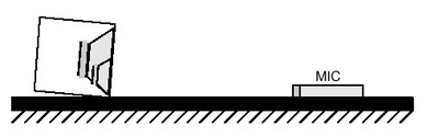
Ground plane method

Ground-plane measurement is commonly used for measuring low-frequency SPL and distortion in subwoofers.

Since it is not representative of free-space radiation, it should not be interpreted as an absolute reference but rather as a comparative measurement method.

Placing the microphone close to the ground makes the direct and reflected sound paths essentially equal in length. The ground therefore acts as an acoustic image source, reinforcing the direct sound. At low frequencies, where the wavelength is large compared with the distance between the real and image sources, the two contributions combine constructively, resulting in an approximately 6 dB increase in SPL compared with free-field radiation.

A correction can be applied if a free-field equivalent level is required.

At higher frequencies, the shorter wavelengths produce frequency-dependent interference between the direct sound and the ground image, resulting in constructive and destructive patterns. This makes the ground-plane method unsuitable for measuring the free-space polar response of a loudspeaker, because the ground image modifies the radiation pattern.

However, the method remains useful for low-frequency SPL and distortion measurements, where the ground-plane configuration provides a controlled and repeatable measurement condition.

Do not underestimate wind, natural noise, or passing vehicles when using this methodology, as they can significantly affect low-frequency measurements.

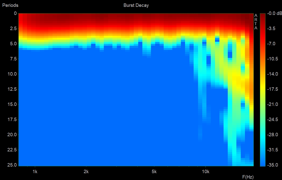
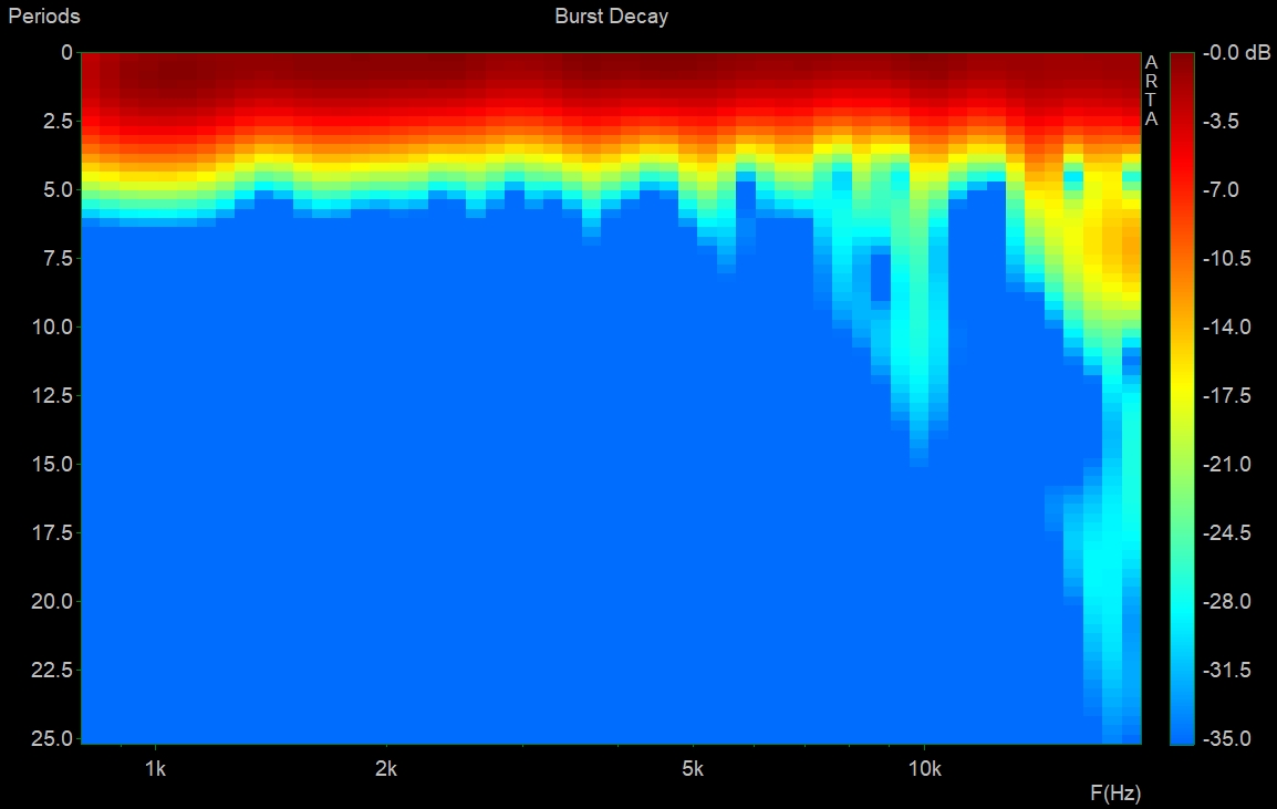
Time domain and breakup impact of polar

Even when normalized, time-domain issues have a significant impact on polar measurements. This is because when a time-domain problem occurs within the driver, due to diaphragm breakup, phase plug anomalies, or other factors, the resulting wavefront deviates from ideal plane wave radiation and no longer perfectly follows the horn profile. This leads to irregularities in the polar response.

If the breakup is well-damped or the time-domain disturbance is minor, the effect remains subtle. However, in the case of severe breakup caused by a rigid diaphragm, the impact becomes much more noticeable. Rigid diaphragms are not inherently bad; they push time-domain issues to higher frequencies compared to softer diaphragms. However, the breakup they introduce is often more abrupt, leading to distinct anomalies in the polar response.

Another point to take into consideration: the more energy (SPL) we send into the breakup region, the more visible the artifacts will be. Therefore, the higher a horn maintains constant directivity at high frequencies, the more the breakup effects will appear on the polar response.

For example:

With a rigid diaphragm driver such as the Faital HF108R:

With a very well-controlled hard diaphragm unit, the 18Sound 1095N:

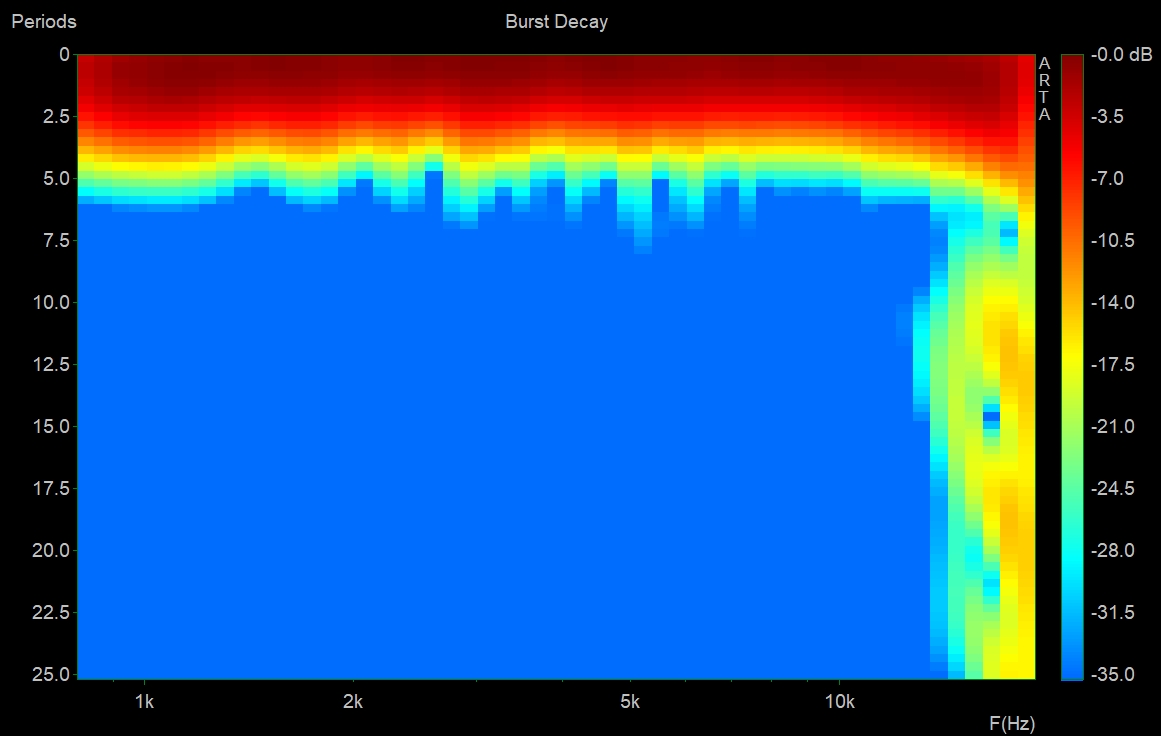
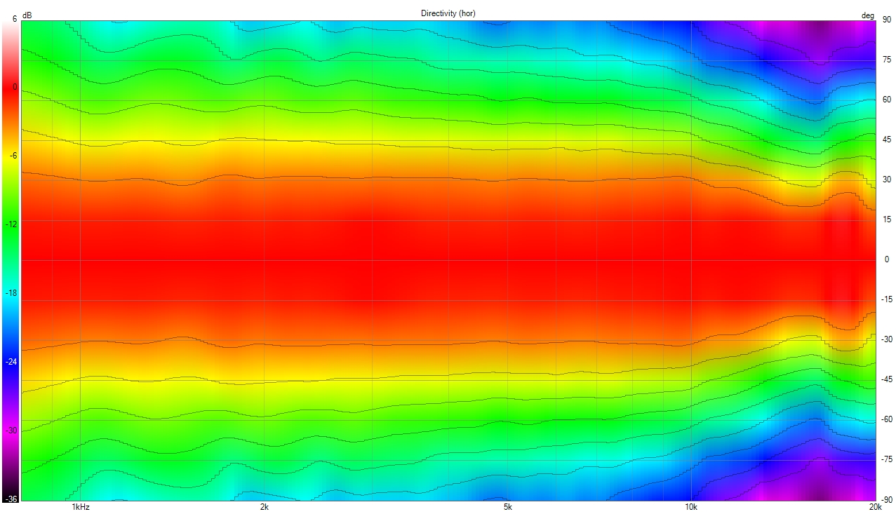
A plastic annular diaphragm, which is less sensitive to breakup due to its shape, the BMS 5530:

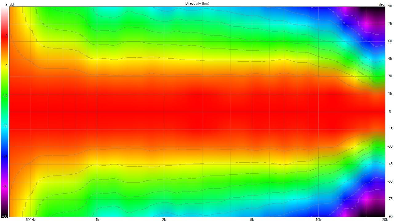
We can see that even when normalized, time-domain behavior has a direct impact on polar measurements due to deviations from perfect plane wave radiation.

Time domain accidents due to the driver have a direct impact on normalized directivity.

Measurement Context

In polar measurements, it is crucial to characterize what we actually want to analyze, the horn, rather than external factors such as the environment or even diaphragm tuning.

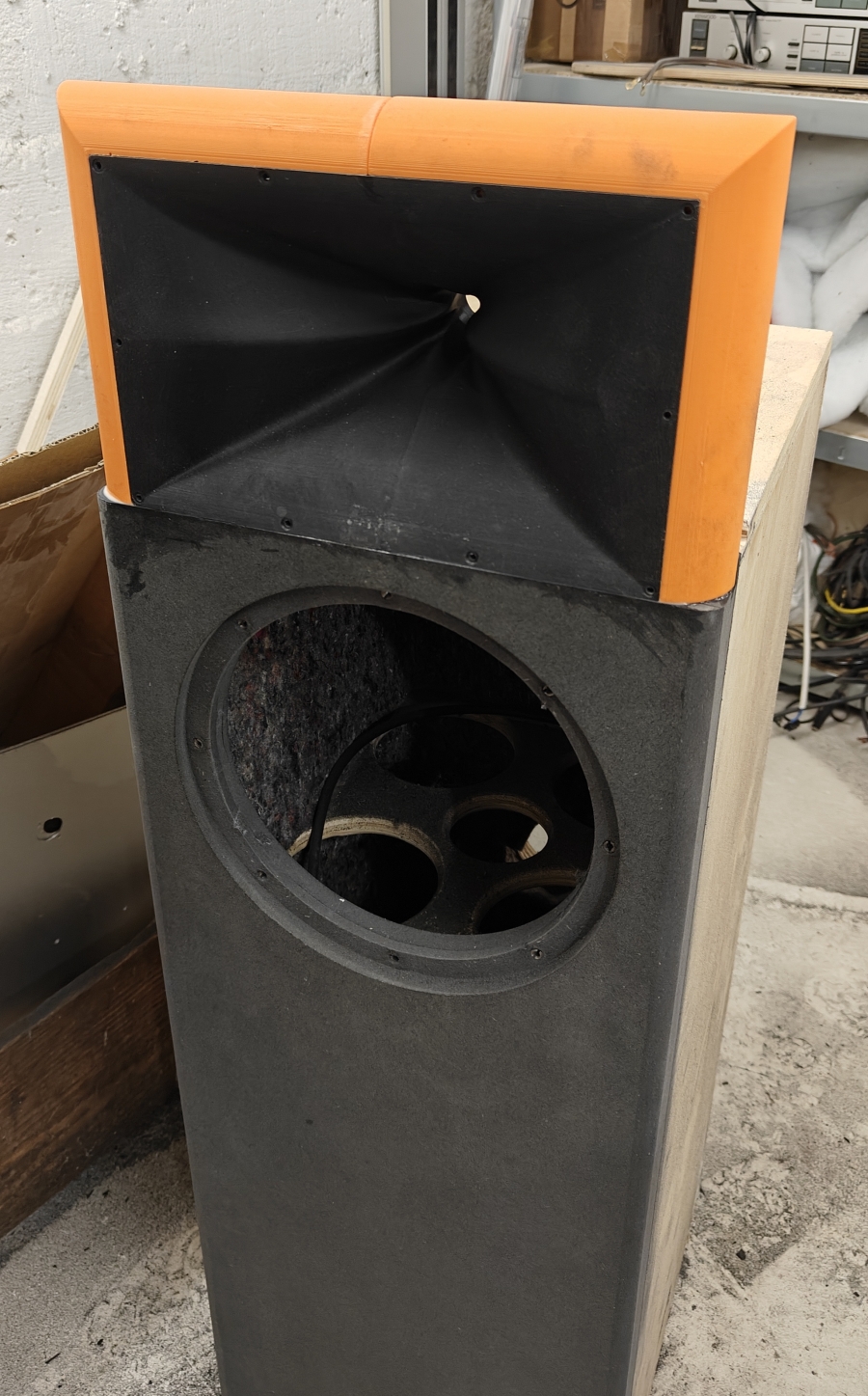
Horn integration

A horn without a roundover should not be measured in free air. When a horn has a fluid profile, such as ours, the best approach is to use the final roundover return that will be used in the speaker, as advised on the website:

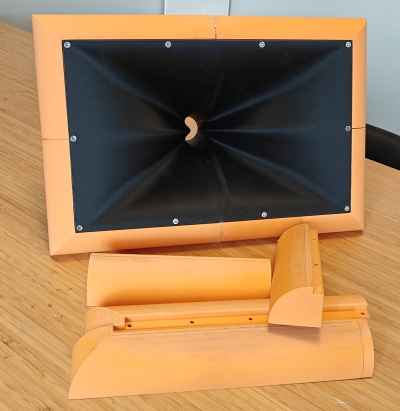
These are very important in measurement and also in the final speaker:

More information about Midrange narrowing and beaming in our dedicated article.

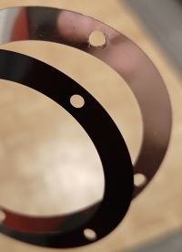
Diaphragm tuning impact

Diaphragm tuning is an important factor in the measurement context, as it can vary even within the same reference. In modern drivers, there are typically two measurements: one for the diaphragm and another for the compression driver.

By subtracting these values and adding adjustment rings of 0.05, 0.1, or 0.2 mm, we can set the proper diaphragm height:

However, this method may not always be precise enough. Some diaphragms are more sensitive to factory tuning variations, with hard diaphragms being far less tolerant to height errors than softer ones.

Below are two measurements of the same compression driver, with normalized polar plots, first with factory tuning and then after retuning by AudioHorn:

We can see a noticeable difference between the two measurements, caused solely by a diaphragm height variation of just 0.05 to 0.1 mm.

Of course, a horn cannot correct driver anomalies, and they will be noticeable on the polar map, even if it is normalized.

Phase Plug can also be at the origin of directivity or/and temporal accident, both often linked.

Room Impact

Except in large anechoic chambers with treated ground and walls, most measurement environments, even with significant quantities of melamine, will have reflective surfaces that introduce irregularities. This can be seen in the impulse response below:

Choosing to measure outdoors can also introduce issues due to the floor and wind conditions.

This is why most measurements are gated. It’s also important to note that our brain dynamically gates measurements, which is what we refer to as ITDG (Impulse Time Delay Gap) or integration time. ITDG is considered to be approximately one cycle (Time = 1/Hz), meaning it varies with frequency.

Woofer physical presence

Whether playing or not, the physical presence of the woofer beneath the horn will mainly affect the vertical polar pattern, but will also affect the horizontal polar pattern. However, the larger the speaker, the less noticeable this impact becomes as the components are further apart.

Mode detail in our diffraction and standing waves article.

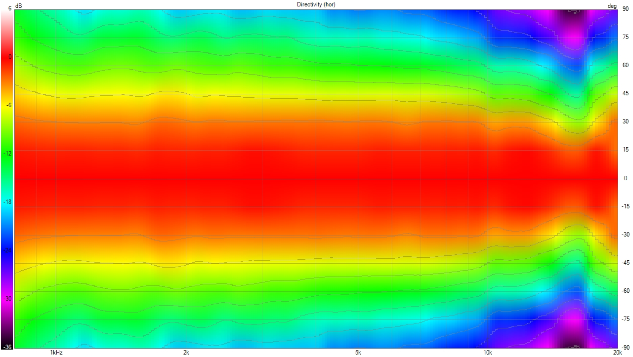
Measurement of first version X25 by clients

Below is an example of several measurements of the X25 old version, the new one is a little bit more straight after 4/5khz :

Client 1:

Conditions:

Inside horn at 2 meters from floor and ceiling
crossed with a mid-woofer at 1300hz
Measuring distance: 2 meters
Round over used: Yes
Degree definition: 10°
Smoothing: 1/12
Gated: Yes
Driver: BMS 4550
APEX respect as turning centering point: Yes
physical presence of woofer: Yes, realistic but alter the horn horizontal polar

Client 2:

Conditions:

Inside horn at 2 meters from floor and ceiling
crossed with a mid-woofer at 1300hz
Measuring distance: 1 meter
Round over used: Yes
Degree definition: 15°
Smoothing: none
Gated: Yes 7ms
Driver: BMS 5530
APEX respect as turning centering point: No, so directivity distotion is on the graph as see upper
physical presence of woofer: Yes, realistic but alter the horn horizontal polar

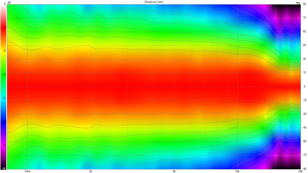
Client 3:

Conditions:

Inside horn at 1 meters from floor
crossed with a mid-woofer at 1250hz
Measuring distance: 1 meters
Round over used: Yes (final speaker)
Degree definition: 15°
Smoothing: 1/24
Gated: Yes 5ms (ground reflection)
Driver: BMS 5530
APEX respect as turning centering point: Yes
physical presence of woofer: Yes, realistic but alter the horn horizontal polar

Conclusion

In conclusion, the measurement methodology is crucial for obtaining accurate and reliable data. However, it is essential to avoid measuring the environment or the measurement setup itself instead of the actual object of analysis, the horn or waveguide. Interpreting the results is key, as we must keep in mind that certain phenomena, such as artifacts from compression drivers, are inevitable and cannot be corrected by the horn.

The compression driver has a direct impact on the results, phase and frequency response anomalies, breakup modes, temporal behavior, and phase plug effects, all of which leave a clear imprint on the polar plots. These effects cannot be eliminated through simple normalization or adjustments to the horn. Therefore, it is essential to account for these imperfections when interpreting the data, rather than attributing them solely to measurement errors or to the horn itself.

A solid methodology ensures that the measurements reflect the system’s actual behavior, not artifacts introduced by the environment or the measurement technique. By following rigorous practices and staying mindful of the specific characteristics of each component, we can obtain useful data for ongoing optimization and better control of directivity, while maintaining a realistic view of the system’s performance.

Sources

A message from Kolbrek about directivity in HornResp:

I believe Hornresp uses a Far-field approximation model for directivity, i.e. that the directivity pattern is calculated as it would appear if you measured it at a very large distance, but the level is scaled back to a 1m distance. Otherwise, you would have to specify a measurement distance and point of rotation, and there would be a large variation in the pattern depending on those values.

If the measurement point is very far away, these variations become insignificant, and the actual rotation point does not matter.

What is “very far away” depends on the size of the source (horn mouth) and also on the “apparent apex” or center of curvature of the far field wave front.

In addition, there are near-field effects. These typically happen when the distance is shorter than (Source area)/(wavelength), this distance is called the Rayleigh distance. At larger distances, the pressure varies as 1/distance, but closer to the source the variations do not follow this law, and have peaks and dips you wouldn’t see at a greater distance.

These effects are usually not a problem when measuring small devices like direct radiators and small horns, but most horns are large enough that they become noticeable, especially at the standard distance of 1m.

When measuring horns, it is usually recommended to rotate them around the “apparent apex”. This will avoid distortion of the directivity pattern at short distances compared to the far-field pattern.

Also note that Hornresp uses one-dimensional horn models, so the directivity models are only approximations.